K-matrix

K-matrix#

While ampform does not yet provide a generic way to formulate an amplitude model with \(\boldsymbol{K}\)-matrix dynamics, the (experimental) kmatrix module makes it fairly simple to produce a symbolic expression for a parameterized \(\boldsymbol{K}\)-matrix with an arbitrary number of poles and channels and play around with it interactively. For more info on the \(\boldsymbol{K}\)-matrix, see the classic paper by Chung [Chung et al., 1995], PDG2021, §Resonances, or this instructive presentation [Meyer, 2008].

Section Physics summarizes [Chung et al., 1995], so that the kmatrix module can reference to the equations. It also points out some subtleties and deviations.

Note

The \(\boldsymbol{K}\)-matrix approach was originally worked worked out in K-matrix, Lorentz-invariant K-matrix, and P-vector. Those reports contained a few mistakes, which have been addressed here.

%matplotlib widget

Physics#

The \(\boldsymbol{K}\)-matrix formalism is used to describe coupled, two-body formation processes of the form \(c_j d_j \to R \to a_i b_i\), with \(i,j\) representing each separate channel and \(R\) an intermediate state by which these channels are coupled.

../../_images/5bd923c2dd46adf5db0ce0fbaca4e1b5d444aabd3e27c4b35129e746fe94bccc.svg

A small adaptation allows us to describe a coupled, two-body production process of the form \(R \to a_ib_i\) (see Production processes).

In the following, \(n\) denotes the number of channels and \(n_R\) the number of poles. In the kmatrix module, we use \(0 \leq i,j < n\) and \(1 \leq R \leq n_R\).

Partial wave expansion#

In amplitude analysis, the main aim is to express the differential cross section \(\frac{d\sigma}{d\Omega}\), that is, the intensity distribution in each spherical direction \(\Omega=(\phi,\theta)\) as we can observe in experiments. This differential cross section can be expressed in terms of the scattering amplitude \(A\):

(1)#\[ \frac{d\sigma}{d\Omega} = \left|A(\Omega)\right|^2. \]

We can now further express \(A\) in terms of partial wave amplitudes by expanding it in terms of its angular momentum components:[1]

(2)#\[ A(\Omega) = \frac{1}{q_i}\sum_L\left(2L+1\right) T_L(s) {D^{*L}_{\lambda\mu}}\left(\phi,\theta,0\right) \]

with \(L\) the total angular momentum of the decay product pair, \(\lambda=\lambda_a-\lambda_b\) and \(\mu=\lambda_c-\lambda_d\) the helicity differences of the final and initial states, \(D\) a Wigner-\(D\) function, and \(T_J\) an operator representing the partial wave amplitude.

The above sketch is just with one channel in mind. The same holds true though for a number of channels \(n\), with the only difference being that the \(T\) operator becomes an \(n\times n\) \(\boldsymbol{T}\)-matrix.

Transition operator#

The important point is that we have now expressed \(A\) in terms of an angular part (depending on \(\Omega\)) and a dynamical part \(\boldsymbol{T}\) that depends on the Mandelstam variable \(s\).

The dynamical part \(\boldsymbol{T}\) is usually called the transition operator. It describes the interacting part of the more general scattering operator \(\boldsymbol{S}\), which describes the (complex) amplitude \(\langle f|\boldsymbol{S}|i\rangle\) of an initial state \(|i\rangle\) transitioning to a final state \(|f\rangle\). The scattering operator describes both the non-interacting amplitude and the transition amplitude, so it relates to the transition operator as:

(3)#\[ \boldsymbol{S} = \boldsymbol{I} + 2i\boldsymbol{T} \]

with \(\boldsymbol{I}\) the identity operator. Just like in [Chung et al., 1995], we use a factor 2, while other authors choose \(\boldsymbol{S} = \boldsymbol{I} + i\boldsymbol{T}\). In that case, one would have to multiply Eq. (2) by a factor \(\frac{1}{2}\).

Ensuring unitarity#

Knowing the origin of the \(\boldsymbol{T}\)-matrix, there is an important restriction that we need to comply with when we further formulate a parametrization: unitarity. This means that \(\boldsymbol{S}\) should conserve probability, namely \(\boldsymbol{S}^\dagger\boldsymbol{S} = \boldsymbol{I}\). Luckily, there is a trick that makes this easier. If we express \(\boldsymbol{S}\) in terms of an operator \(\boldsymbol{K}\) by applying a Cayley transformation:

(4)#\[ \boldsymbol{S} = (\boldsymbol{I} + i\boldsymbol{K})(I - i\boldsymbol{K})^{-1}, \]

unitarity is conserved if \(\boldsymbol{K}\) is real. With some matrix jumbling, we can derive that the \(\boldsymbol{T}\)-matrix can be expressed in terms of \(\boldsymbol{K}\) as follows:

(5)#\[ \boldsymbol{T} = \boldsymbol{K} \left(\boldsymbol{I} - i\boldsymbol{K}\right)^{-1} = \left(\boldsymbol{I} - i\boldsymbol{K}\right)^{-1} \boldsymbol{K}. \]

Lorentz-invariance#

The description so far did not take Lorentz-invariance into account. For this, we first need to define a two-body phase space matrix \(\boldsymbol{\rho}\):

(6)#\[\begin{split} \boldsymbol{\rho} = \begin{pmatrix} \rho_0 & \cdots & 0 \\ \vdots & \ddots & \vdots \\ 0 & \cdots & \rho_{n-1} \end{pmatrix}. \end{split}\]

with \(\rho_i\) given by (1) in PhaseSpaceFactor for the final state masses \(m_{a,i}, m_{b,i}\). The Lorentz-invariant amplitude \(\boldsymbol{\hat{T}}\) and corresponding Lorentz-invariant \(\boldsymbol{\hat{K}}\)-matrix can then be computed from \(\boldsymbol{T}\) and \(\boldsymbol{K}\) with:[2]

(7)#\[\begin{split} \begin{eqnarray} \boldsymbol{T} & = & \sqrt{\boldsymbol{\rho}} \; \boldsymbol{\hat{T}} \sqrt{\boldsymbol{\rho}} \\ \boldsymbol{K} & = & \sqrt{\boldsymbol{\rho}} \; \boldsymbol{\hat{K}} \sqrt{\boldsymbol{\rho}}. \end{eqnarray} \end{split}\]

With these definitions, we can deduce that:

(8)#\[ \boldsymbol{\hat{T}} = \boldsymbol{\hat{K}} (\boldsymbol{I} - i\boldsymbol{\rho}\boldsymbol{\hat{K}})^{-1} = (\boldsymbol{I} - i\boldsymbol{\hat{K}}\boldsymbol{\rho})^{-1} \boldsymbol{\hat{K}}. \]

Production processes#

As noted in the intro, the \(\boldsymbol{K}\)-matrix describes scattering processes of type \(cd \to ab\). It can however be generalized to describe production processes of type \(R \to ab\). Here, the amplitude is described by a final state \(F\)-vector of size \(n\), so the question is how to express \(F\) in terms of transition matrix \(\boldsymbol{T}\).

../../_images/712016e0c53056c4c98c21ec70183f51f626e11001658f3fb181346a913d977e.svg

One approach by [Aitchison, 1972] is to transform \(\boldsymbol{T}\) into \(F\) (and its relativistic form \(\hat{F}\)) through the production amplitude \(P\)-vector:

(9)#\[\begin{split} \begin{eqnarray} F & = & \left(\boldsymbol{I}-i\boldsymbol{K}\right)^{-1}P \\ \hat{F} & = & \left(\boldsymbol{I}-i\boldsymbol{\hat{K}\boldsymbol{\rho}}\right)^{-1}\hat{P}, \end{eqnarray} \end{split}\]

where we can compute \(\boldsymbol{\hat{K}}\) from (7):

(10)#\[ \hat{\boldsymbol{K}} = \sqrt{\boldsymbol{\rho}^{-1}} \boldsymbol{K} \sqrt{\boldsymbol{\rho}^{-1}}. \]

Another approach by [Cahn and Landshoff, 1986] further approximates this by defining a \(Q\)-vector:

(11)#\[ Q = \boldsymbol{K}^{-1}P \quad \mathrm{and} \quad \hat{Q} = \boldsymbol{\hat{K}}^{-1}\hat{P} \]

that is taken to be constant (just some ‘fitting’ parameters). The \(F\)-vector can then be expressed as:

(12)#\[ F = \boldsymbol{T}Q \quad \mathrm{and} \quad \hat{F} = \boldsymbol{\hat{T}}\hat{Q} \]

Note that for all these vectors, we have:

(13)#\[ F=\sqrt{\boldsymbol{\rho}}\hat{F},\quad P=\sqrt{\boldsymbol{\rho}}\hat{P},\quad\mathrm{and}\quad Q=\sqrt{\boldsymbol{\rho}^{-1}}\hat{Q}. \]

Pole parametrization#

After all these matrix definitions, the final challenge is to choose a correct parametrization for the elements of \(\boldsymbol{K}\) and \(P\) that accurately describes the resonances we observe.[3] There are several choices, but a common one is the following summation over the poles \(R\):[4]

(14)#\[\begin{split} \begin{eqnarray} K_{ij} &=& \sum_R\frac{g_{R,i}g_{R,j}}{m_R^2-s} + c_{ij} \\ \hat{K}_{ij} &=& \sum_R \frac{g_{R,i}(s)g_{R,j}(s)}{\left(m_R^2-s\right)\sqrt{\rho_i\rho_j}} + \hat{c}_{ij} \end{eqnarray} \end{split}\]

with \(c_{ij}, \hat{c}_{ij}\) some optional background characterization and \(g_{R,i}\) the residue functions. The residue functions are often further expressed as:

(15)#\[\begin{split} \begin{eqnarray} g_{R,i} &=& \gamma_{R,i}\sqrt{m_R\Gamma^0_{R,i}} \\ g_{R,i}(s) &=& \gamma_{R,i}\sqrt{m_R\Gamma_{R,i}(s)} \end{eqnarray} \end{split}\]

with \(\gamma_{R,i}\) some real constants and \(\Gamma^0_{R,i}\) the partial width of each pole. In the Lorentz-invariant form, the fixed width \(\Gamma^0\) is replaced by an “energy dependent” EnergyDependentWidth \(\Gamma(s)\).[5] The width for each pole can be computed as \(\Gamma^0_R = \sum_i\Gamma^0_{R,i}\).

The production vector \(P\) is commonly parameterized as:[6]

(16)#\[\begin{split} \begin{eqnarray} P_i &=& \sum_R \frac{\beta^0_R\,g_{R,i}(s)}{m_R^2-s} \\ \hat{P}_i &=& \sum_R \frac{\beta^0_R\,g_{R,i}(s)}{\left(m_R^2-s\right)\sqrt{\rho_i}} \\ &=& \sum_R \frac{ \beta^0_R\gamma_{R,i}m_R\Gamma^0_R B_{R,i}(q(s)) }{m_R^2-s} \end{eqnarray} \end{split}\]

with \(B_{R,i}(q(s))\) the centrifugal damping factor (see FormFactor and BlattWeisskopfSquared) for channel \(i\) and \(\beta_R^0\) some (generally complex) constants that describe the production information of the decaying state \(R\). Usually, these constants are rescaled just like the residue functions in (15):

(17)#\[ \beta^0_R = \beta_R\sqrt{m_R\Gamma^0_R}. \]

Implementation#

Non-relativistic K-matrix#

A non-relativistic \(\boldsymbol{K}\)-matrix for an arbitrary number of channels and an arbitrary number of poles can be formulated with the NonRelativisticKMatrix.formulate() method:

n_poles = sp.Symbol("n_R", integer=True, positive=True)
k_matrix_nr = kmatrix.NonRelativisticKMatrix.formulate(n_poles=n_poles, n_channels=1)
k_matrix_nr[0, 0]

\[\displaystyle \frac{i \sum_{R=1}^{n_{R}} \frac{{\Gamma}_{R,0} {\gamma}_{R,0}^{2} {m}_{R}}{- s + {m}_{R}^{2}}}{\sum_{R=1}^{n_{R}} \frac{{\Gamma}_{R,0} {\gamma}_{R,0}^{2} {m}_{R}}{- s + {m}_{R}^{2}} + i}\]

Notice how the \(\boldsymbol{K}\)-matrix reduces to a relativistic_breit_wigner() in the case of one channel and one pole (but for a residue constant \(\gamma\)):

k_matrix_1r = kmatrix.NonRelativisticKMatrix.formulate(n_poles=1, n_channels=1)
k_matrix_1r[0, 0].doit().simplify()

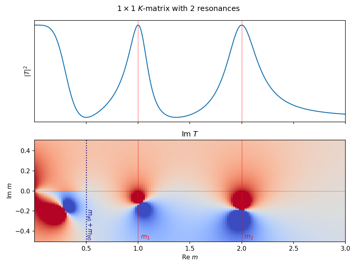
\[\displaystyle - \frac{{\Gamma}_{1,0} {\gamma}_{1,0}^{2} {m}_{1}}{s + i {\Gamma}_{1,0} {\gamma}_{1,0}^{2} {m}_{1} - {m}_{1}^{2}}\]

Now let’s investigate the effect of using a \(\boldsymbol{K}\)-matrix to describe two poles in one channel and see how it compares with the sum of two Breit-Wigner functions (two ‘resonances’). Two Breit-Wigner ‘poles’ with the same parameters would look like this:

s, m1, m2, Gamma1, Gamma2 = sp.symbols("s m1 m2 Gamma1 Gamma2", nonnegative=True)
bw1 = relativistic_breit_wigner(s, m1, Gamma1)
bw2 = relativistic_breit_wigner(s, m2, Gamma2)
bw = bw1 + bw2
bw

\[\displaystyle \frac{\Gamma_{1} m_{1}}{- i \Gamma_{1} m_{1} + m_{1}^{2} - s} + \frac{\Gamma_{2} m_{2}}{- i \Gamma_{2} m_{2} + m_{2}^{2} - s}\]

while a \(\boldsymbol{K}\)-matrix parametrizes the two poles as:

k_matrix_2r = kmatrix.NonRelativisticKMatrix.formulate(n_poles=2, n_channels=1)
k_matrix = k_matrix_2r[0, 0].doit()

\[\displaystyle \frac{i {\Gamma}_{2,0} {\gamma}_{2,0}^{2} {m}_{2}}{\left(- s + {m}_{2}^{2}\right) \left(i + \frac{{\Gamma}_{2,0} {\gamma}_{2,0}^{2} {m}_{2}}{- s + {m}_{2}^{2}} + \frac{{\Gamma}_{1,0} {\gamma}_{1,0}^{2} {m}_{1}}{- s + {m}_{1}^{2}}\right)} + \frac{i {\Gamma}_{1,0} {\gamma}_{1,0}^{2} {m}_{1}}{\left(- s + {m}_{1}^{2}\right) \left(i + \frac{{\Gamma}_{2,0} {\gamma}_{2,0}^{2} {m}_{2}}{- s + {m}_{2}^{2}} + \frac{{\Gamma}_{1,0} {\gamma}_{1,0}^{2} {m}_{1}}{- s + {m}_{1}^{2}}\right)}\]

To simplify things, we can set the residue constants \(\gamma\) to one. Notice how the \(\boldsymbol{K}\)-matrix has introduced some coupling (‘interference’) between the two terms.

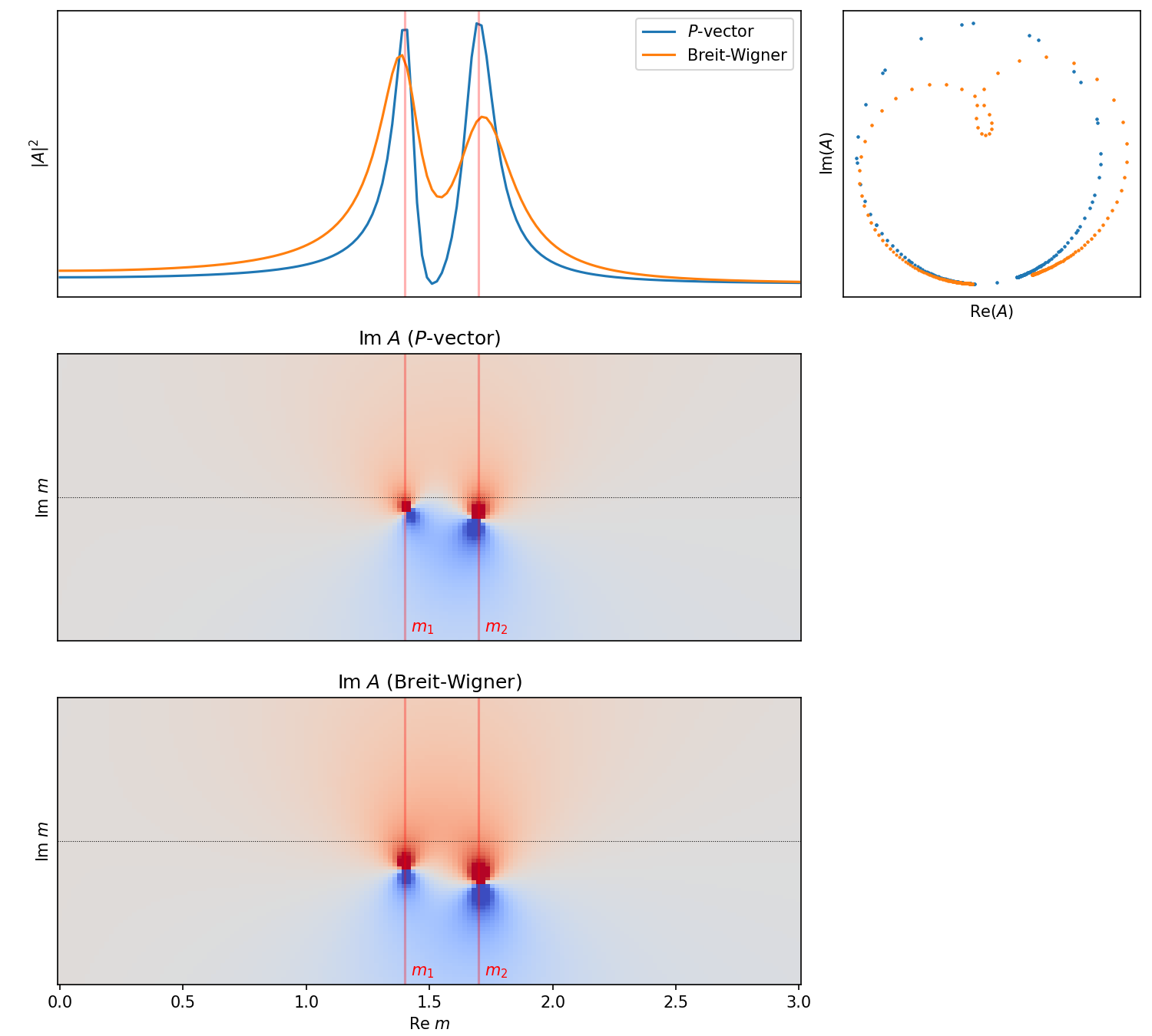
\[\displaystyle \frac{\Gamma_{1} m_{1}}{- i \Gamma_{1} m_{1} + m_{1}^{2} - s} + \frac{\Gamma_{2} m_{2}}{- i \Gamma_{2} m_{2} + m_{2}^{2} - s}\]

\[\displaystyle \frac{i \Gamma_{1,0} m_{1}}{\left(m_{1}^{2} - s\right) \left(\frac{\Gamma_{1,0} m_{1}}{m_{1}^{2} - s} + \frac{\Gamma_{2,0} m_{2}}{m_{2}^{2} - s} + i\right)} + \frac{i \Gamma_{2,0} m_{2}}{\left(m_{2}^{2} - s\right) \left(\frac{\Gamma_{1,0} m_{1}}{m_{1}^{2} - s} + \frac{\Gamma_{2,0} m_{2}}{m_{2}^{2} - s} + i\right)}\]

Now, just like in Inspect model interactively, we use symplot to visualize the difference between the two expressions. The important thing is that the Argand plot on the right shows that the \(\boldsymbol{K}\)-matrix conserves unitarity.

Note that we have to call symplot.substitute_indexed_symbols() to turn the Indexed instances in this Matrix expression into Symbols before calling this function. We also call symplot.rename_symbols() so that the residue \(\gamma\)’s get a name that does not have to be dummified by lambdify().

Show code cell source

Hide code cell source

# Prepare expressions
m = sp.Symbol("m", nonnegative=True)
k_matrix = symplot.substitute_indexed_symbols(k_matrix)
rename_gammas = lambda s: re.sub(  # noqa: E731
    r"\\([Gg])amma_{([0-9]),0}", r"\1amma\2", s
)
gamma1, gamma2 = sp.symbols("gamma1 gamma2", nonnegative=True)
bw = symplot.rename_symbols(bw, rename_gammas)
k_matrix = symplot.rename_symbols(k_matrix, rename_gammas)
bw = bw.xreplace({s: m**2})
k_matrix = k_matrix.xreplace({s: m**2})

# Prepare sliders and domain
np_kmatrix, sliders = symplot.prepare_sliders(k_matrix, m)
np_bw = sp.lambdify((m, Gamma1, Gamma2, gamma1, gamma2, m1, m2), bw.doit())

m_min, m_max = 0, 3
domain_1d = np.linspace(m_min, m_max, 200)
domain_argand = np.linspace(m_min - 2, m_max + 2, 1_000)
sliders.set_ranges(
    m1=(0, 3, 100),
    m2=(0, 3, 100),
    Gamma1=(0, 2, 100),
    Gamma2=(0, 2, 100),
    gamma1=(0, 2),
    gamma2=(0, 2),
)
sliders.set_values(
    m1=1.1,
    m2=1.9,
    Gamma1=0.2,
    Gamma2=0.3,
    gamma1=1,
    gamma2=1,
)
if STATIC_WEB_PAGE:
    # Concatenate flipped domain for reverse animation
    domain = np.linspace(1.0, 2.7, 50)
    domain = np.concatenate((domain, np.flip(domain[1:])))
    sliders._sliders["m1"] = domain


def create_argand(func):
    def wrapped(**kwargs):
        values = func(domain_argand, **kwargs)
        argand = np.array([values.real, values.imag])
        return argand.T

    return wrapped


# Create figure
fig, axes = plt.subplots(
    ncols=2,
    figsize=1.2 * np.array((8, 3.8)),
    tight_layout=True,
)
ax_intensity, ax_argand = axes
m_label = "$m_{a+b}$"
ax_intensity.set_xlabel(m_label)
ax_intensity.set_ylabel("$|A|^2$")
ax_argand.set_xlabel("Re($A$)")
ax_argand.set_ylabel("Im($A$)")

# Plot intensity
controls = iplt.plot(
    domain_1d,
    lambda *args, **kwargs: np.abs(np_kmatrix(*args, **kwargs) ** 2),
    label="$K$-matrix",
    **sliders,
    ylim="auto",
    ax=ax_intensity,
)
iplt.plot(
    domain_1d,
    lambda *args, **kwargs: np.abs(np_bw(*args, **kwargs) ** 2),
    label="Breit-Wigner",
    controls=controls,
    ylim="auto",
    ax=ax_intensity,
)
plt.legend(loc="upper right")
iplt.axvline(controls["m1"], c="gray", linestyle="dotted")
iplt.axvline(controls["m2"], c="gray", linestyle="dotted")

# Argand plots
iplt.scatter(
    create_argand(np_kmatrix),
    label="$K$-matrix",
    controls=controls,
    parametric=True,
    s=1,
    ax=ax_argand,
)
iplt.scatter(
    create_argand(np_bw),
    label="Breit-Wigner",
    controls=controls,
    parametric=True,
    s=1,
    ax=ax_argand,
)
plt.legend(loc="upper right");

../../_images/6ceedb72b756250b082987c40745e983476b206b267d347e1fb9525e2b13b2d3.png

Relativistic K-matrix#

Relativistic \(\boldsymbol{K}\)-matrices for an arbitrary number of channels and an arbitrary number of poles can be formulated with the RelativisticKMatrix.formulate() method:

L = sp.Symbol("L", integer=True, negative=False)
n_poles = sp.Symbol("n_R", integer=True, positive=True)
rel_k_matrix_nr = kmatrix.RelativisticKMatrix.formulate(
    n_poles=n_poles, n_channels=1, angular_momentum=L
)
rel_k_matrix_nr[0, 0]

\[\displaystyle \frac{i \overline{\sqrt{\rho\left(s\right)}} \sqrt{\rho\left(s\right)} \sum_{R=1}^{n_{R}} \frac{\Gamma\left(s\right) {\gamma}_{R,0}^{2} {m}_{R}}{- s + {m}_{R}^{2}}}{\rho\left(s\right) \sum_{R=1}^{n_{R}} \frac{\Gamma\left(s\right) {\gamma}_{R,0}^{2} {m}_{R}}{- s + {m}_{R}^{2}} + i}\]

Again, as in Non-relativistic K-matrix, the \(\boldsymbol{K}\)-matrix reduces to something of a relativistic_breit_wigner(). This time, the width has been replaced by a EnergyDependentWidth and some PhaseSpaceFactors have been inserted that take care of the decay into two decay products:

rel_k_matrix_1r = kmatrix.RelativisticKMatrix.formulate(
    n_poles=1, n_channels=1, angular_momentum=L
)
symplot.partial_doit(rel_k_matrix_1r[0, 0], sp.Sum).simplify(doit=False)

\[\displaystyle - \frac{\overline{\sqrt{\rho\left(s\right)}} \Gamma_{1,0}\left(s\right) {\gamma}_{1,0}^{2} {m}_{1} \sqrt{\rho\left(s\right)}}{s + i \Gamma_{1,0}\left(s\right) {\gamma}_{1,0}^{2} {m}_{1} \rho\left(s\right) - {m}_{1}^{2}}\]

Note that another difference with relativistic_breit_wigner_with_ff() is an additional phase space factor in the denominator. That one disappears in P-vector.

The \(\boldsymbol{K}\)-matrix with two poles becomes (neglecting the \(\sqrt{\rho_0(s)}\)):

rel_k_matrix_2r = kmatrix.RelativisticKMatrix.formulate(
    n_poles=2, n_channels=1, angular_momentum=L
)
rel_k_matrix_2r = symplot.partial_doit(rel_k_matrix_2r[0, 0], sp.Sum)

\[\displaystyle \frac{i \gamma_{1,0}^{2} m_{1} \Gamma_{1,0}\left(s\right)}{\left(m_{1}^{2} - s\right) \left(\left(\frac{\gamma_{1,0}^{2} m_{1} \Gamma_{1,0}\left(s\right)}{m_{1}^{2} - s} + \frac{\gamma_{2,0}^{2} m_{2} \Gamma_{2,0}\left(s\right)}{m_{2}^{2} - s}\right) \rho\left(s\right) + i\right)} + \frac{i \gamma_{2,0}^{2} m_{2} \Gamma_{2,0}\left(s\right)}{\left(m_{2}^{2} - s\right) \left(\left(\frac{\gamma_{1,0}^{2} m_{1} \Gamma_{1,0}\left(s\right)}{m_{1}^{2} - s} + \frac{\gamma_{2,0}^{2} m_{2} \Gamma_{2,0}\left(s\right)}{m_{2}^{2} - s}\right) \rho\left(s\right) + i\right)}\]

This again shows the interference introduced by the \(\boldsymbol{K}\)-matrix, when compared with a sum of two Breit-Wigner functions.

P-vector#

For one channel and an arbitrary number of poles \(n_R\), the \(F\)-vector gets the following form:

n_poles = sp.Symbol("n_R", integer=True, positive=True)
kmatrix.NonRelativisticPVector.formulate(n_poles=n_poles, n_channels=1)[0]

\[\displaystyle \frac{i \sum_{R=1}^{n_{R}} \frac{{\Gamma}_{R,0} {\beta}_{R} {\gamma}_{R,0} {m}_{R}}{- s + {m}_{R}^{2}}}{\sum_{R=1}^{n_{R}} \frac{{\Gamma}_{R,0} {\gamma}_{R,0}^{2} {m}_{R}}{- s + {m}_{R}^{2}} + i}\]

The RelativisticPVector looks like:

kmatrix.RelativisticPVector.formulate(
    n_poles=n_poles, n_channels=1, angular_momentum=L
)[0]

\[\displaystyle \frac{\overline{\sqrt{\rho\left(s\right)}} \sqrt{\rho\left(s\right)} \sum_{R=1}^{n_{R}} \frac{\mathcal{F}_{L}\left(s, {m_{a}}_{0}, {m_{b}}_{0}\right) {\Gamma}_{R,0} {\beta}_{R} {\gamma}_{R,0} {m}_{R}}{- s + {m}_{R}^{2}}}{\overline{\sqrt{\rho\left(s\right)}} - i \sqrt{\rho\left(s\right)} \sum_{R=1}^{n_{R}} \frac{\Gamma\left(s\right) {\gamma}_{R,0}^{2} {m}_{R}}{- s + {m}_{R}^{2}}}\]

As in Non-relativistic K-matrix, if we take \(n_R=1\), the \(F\)-vector reduces to a Breit-Wigner function, but now with an additional factor \(\beta\).

f_vector_1r = kmatrix.NonRelativisticPVector.formulate(n_poles=1, n_channels=1)
symplot.partial_doit(f_vector_1r[0], sp.Sum)

\[\displaystyle \frac{i {\Gamma}_{1,0} {\beta}_{1} {\gamma}_{1,0} {m}_{1}}{\left(i + \frac{{\Gamma}_{1,0} {\gamma}_{1,0}^{2} {m}_{1}}{- s + {m}_{1}^{2}}\right) \left(- s + {m}_{1}^{2}\right)}\]

And when we neglect the phase space factors \(\sqrt{\rho_0(s)}\), the RelativisticPVector reduces to a relativistic_breit_wigner_with_ff()!

rel_f_vector_1r = kmatrix.RelativisticPVector.formulate(
    n_poles=1, n_channels=1, angular_momentum=L
)
rel_f_vector_1r = symplot.partial_doit(rel_f_vector_1r[0], sp.Sum)

\[\displaystyle - \frac{\Gamma_{1,0} \gamma_{1,0} \beta_{1} m_{1} \mathcal{F}_{L}\left(s, m_{a0}, m_{b0}\right)}{i \gamma_{1,0}^{2} m_{1} \Gamma_{1,0}\left(s\right) - m_{1}^{2} + s}\]

Note that the \(F\)-vector approach introduces additional \(\beta\)-coefficients. These can constants can be complex and can introduce phase differences form the production process.

f_vector_2r = kmatrix.NonRelativisticPVector.formulate(n_poles=2, n_channels=1)
f_vector = f_vector_2r[0].doit()

\[\displaystyle \frac{i {\Gamma}_{2,0} {\beta}_{2} {\gamma}_{2,0} {m}_{2}}{\left(- s + {m}_{2}^{2}\right) \left(i + \frac{{\Gamma}_{2,0} {\gamma}_{2,0}^{2} {m}_{2}}{- s + {m}_{2}^{2}} + \frac{{\Gamma}_{1,0} {\gamma}_{1,0}^{2} {m}_{1}}{- s + {m}_{1}^{2}}\right)} + \frac{i {\Gamma}_{1,0} {\beta}_{1} {\gamma}_{1,0} {m}_{1}}{\left(- s + {m}_{1}^{2}\right) \left(i + \frac{{\Gamma}_{2,0} {\gamma}_{2,0}^{2} {m}_{2}}{- s + {m}_{2}^{2}} + \frac{{\Gamma}_{1,0} {\gamma}_{1,0}^{2} {m}_{1}}{- s + {m}_{1}^{2}}\right)}\]

Now again let’s compare the compare this with a sum of two relativistic_breit_wigner()s, now with the two additional \(\beta\)-constants.

beta1, beta2 = sp.symbols("beta1 beta2", nonnegative=True)
bw_with_phases = beta1 * bw1 + beta2 * bw2
display(
    bw_with_phases,
    remove_residue_constants(f_vector),
)

\[\displaystyle \frac{\Gamma_{1} \beta_{1} m_{1}}{- i \Gamma_{1} m_{1} + m_{1}^{2} - s} + \frac{\Gamma_{2} \beta_{2} m_{2}}{- i \Gamma_{2} m_{2} + m_{2}^{2} - s}\]

\[\displaystyle \frac{i \Gamma_{1,0} \beta_{1} m_{1}}{\left(m_{1}^{2} - s\right) \left(\frac{\Gamma_{1,0} m_{1}}{m_{1}^{2} - s} + \frac{\Gamma_{2,0} m_{2}}{m_{2}^{2} - s} + i\right)} + \frac{i \Gamma_{2,0} \beta_{2} m_{2}}{\left(m_{2}^{2} - s\right) \left(\frac{\Gamma_{1,0} m_{1}}{m_{1}^{2} - s} + \frac{\Gamma_{2,0} m_{2}}{m_{2}^{2} - s} + i\right)}\]